VideoDB Documentation

Pages

How VideoDB Solves Complex Visual Analysis Tasks

Vision Language Models (VLMs) shine in controlled benchmarks, yet they stumble in real-world, event-dense footage such as an NFL game. VideoDB bridges that gap by letting developers slice video at the right semantic boundaries, combine external stats, and run multi-tier visual/LLM pipelines that cut hallucinations by >80 % while costing up to 70 % less than a naïve “1 fps into Gemini” workflow. If you need fast, cheap, accurate visual reasoning, you need more than a big VLM—you need a video-native AI Infrastructure.

In this blog, we’ll explore different basic to advance approaches for

NFL game footage.⁠

We want this writeup to guide you into solving real world scenarios in video understanding. To know how each method performed, we focused on following key aspects:

Hallucination

Frequency of incorrect or irrelevant information produced by the VLM.

Temporal Context

How accurately the VLM maintains correct chronological relationships within the video.

Performance on Granular Queries

The VLM's effectiveness in accurately responding to detailed and specific queries.

VideoDB Involvement

The extent to which VideoDB's capabilities were leveraged to enhance VLM performance

There are no rows in this table

⁠

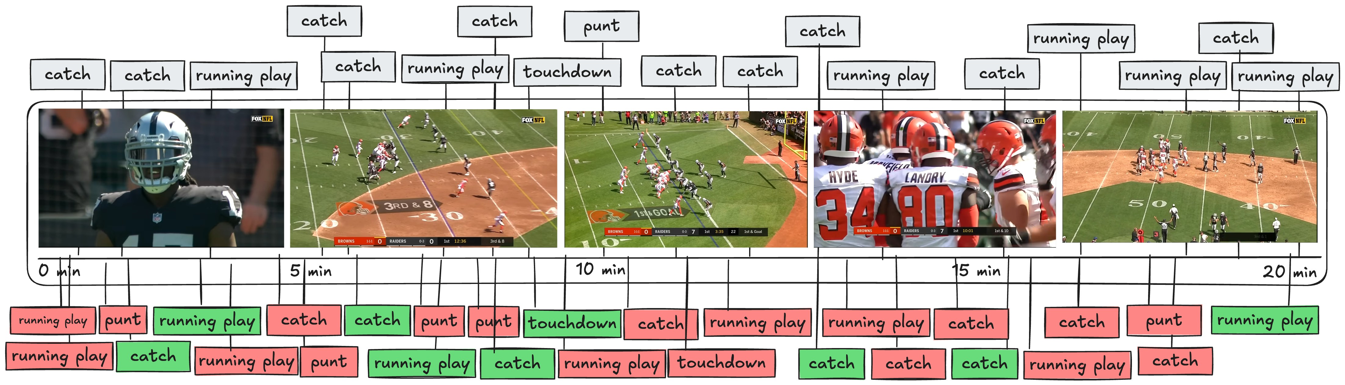
1- The Naive Gemini Approach

⁠

Initially, we tried directly inputting complete NFL game footage into Gemini, expecting robust results based on benchmark promises.

Observations

Evaluation metric

Observation

Notes

Hallucination

68.1 %

Frequent irrelevant predictions (68.1%).

Temporal Context

Bloated

Model often lost critical event continuity.

Performance on Granular Queries

Moderate

Struggled significantly.

VideoDB Involvement

Low

There are no rows in this table

⁠

The model frequently produced incorrect or imaginary events (hallucinations), and misclassifications were common. Furthermore, it often completely missed or overlooked critical events, revealing significant weaknesses in accuracy and contextual comprehension

⁠

This visualization shows a timeline of the first 20 minutes of the game. The top row in grey indicates the ground truth (actual events from the game), while the bottom row displays predictions made by VLM. Each predicted label is color coded: green indicates the model correctly matched the ground truth, and red indicates a mismatch. This side by side comparison helps assess the VLM’s performance. For this visualization, we have limited the scope to running plays, catches, touchdowns, and punts.

Known VLM Limitations (Why “just send it to Gemini” falls short)

Finite context windows – even a 1 M-token window can’t hold one NFL quarter at 30 fps.

Image-tile token explosion – every 1080p frame is split into ~4–9 tiles (≈ 1–4 k tokens) before the model “sees” it.

Weak event reasoning – current VLMs reason per-frame, not per-play; they miss temporal causality (e.g., “Was the QB still behind the line when he released?”).

Cost scales linearly with frames, so 30 fps steals wallets fast.

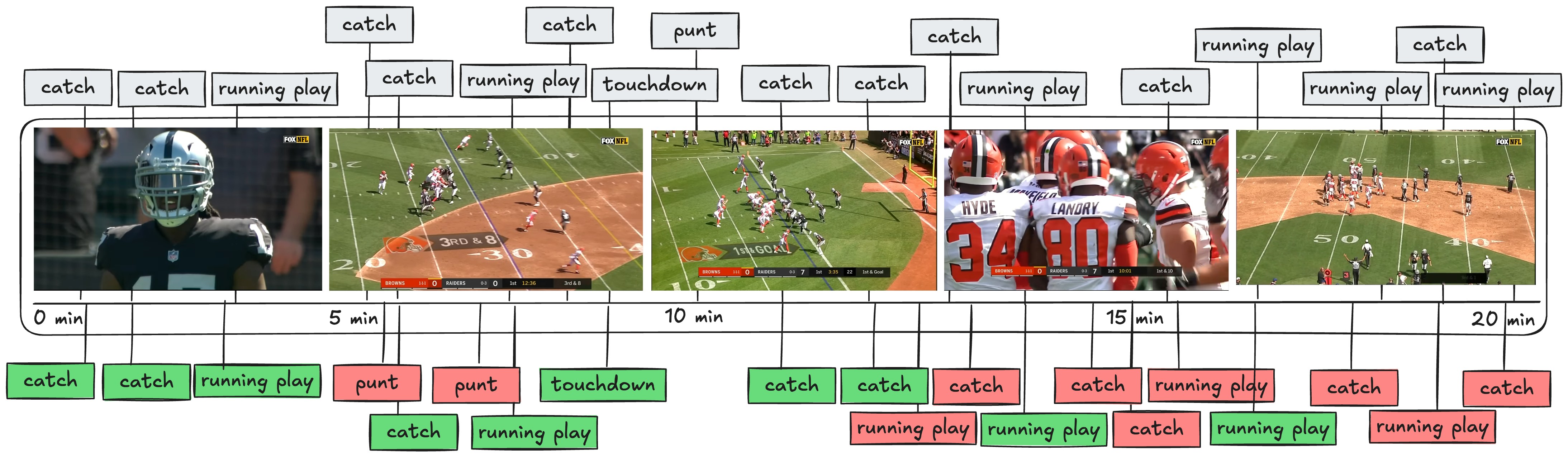
2. Uniform-Length Chunks ( Possible with VideoDB)

⁠

We chopped footage into fixed 2 s / 5 s / 10 s clips via VideoDB’s scene index API. The hypothesis was straightforward: shorter, consistently sized segments might simplify the VLM’s task, potentially enhancing accuracy.

Code snippet for uniform chunk segmentation:

from videodb import SceneExtractionType

conn = videodb.connect(api_key="YOUR_API_KEY")

collection = conn.get_collection()

video = collection.upload(url="https://www.youtube.com/...")

# Extract uniform scenes every n seconds

scene_collection = video.extract_scenes(

extraction_type=SceneExtractionType.time_based,

extraction_config={"time": 5, "num_frames": 150}, # Example: 5 seconds per chunk

)

print(f"Scene Collection ID: {scene_collection.id}")

The goal of testing these configurations was to understand how varying segment lengths could impact model accuracy and output clarity.

Observations

Evaluation metric

Observation

Hallucination

74.2 %

Temporal Context

Insufficient

Performance on Granular Queries

Moderate

VideoDB Involvement

Moderate

There are no rows in this table

⁠

Arbitrary clip boundaries lose context

Important actions (e.g., QB throw) get split across two clips, so the model can’t see the full play and mis-judges legality or outcome.

Same problem pops up for catches, interceptions, and other decisive moments.

Higher hallucination rate

Model starts “imagining” passes and catches that never happened, simply because it lacks enough temporal evidence in a single clip.

Resulting event timeline is noisy and bloated with false positives.

Goldilocks problem with clip length

Too long → information overload and confusion.

Too short → not enough context.

Neither extreme works; we need a balanced segmentation window.

3. Play-by-Play Segmentation ( Advanced Pipeline with VideoDB)

During our analysis, we found that detailed statistical reports for major sports games are typically publicly available. These reports offer extensive information ranging from basic team formations and player lineups to precise, event-specific details such as passes, touchdowns, interceptions, and catches. Most importantly for our analysis, these reports include exact timestamps marking the start and end of each play, making them ideal for accurate segmentation.

Reliable sources for such detailed play-by-play data include official NFL Scores pages, where users can select specific seasons, weeks, and games to access comprehensive statistics. For our specific analysis, we referred directly to the official game summary PDF.

However, we encountered a significant practical issue: the timestamps provided by these reports reflected the official game clock, not the actual video timestamps. To segment the video correctly, we needed to align these official game timestamps accurately with the video's runtime.

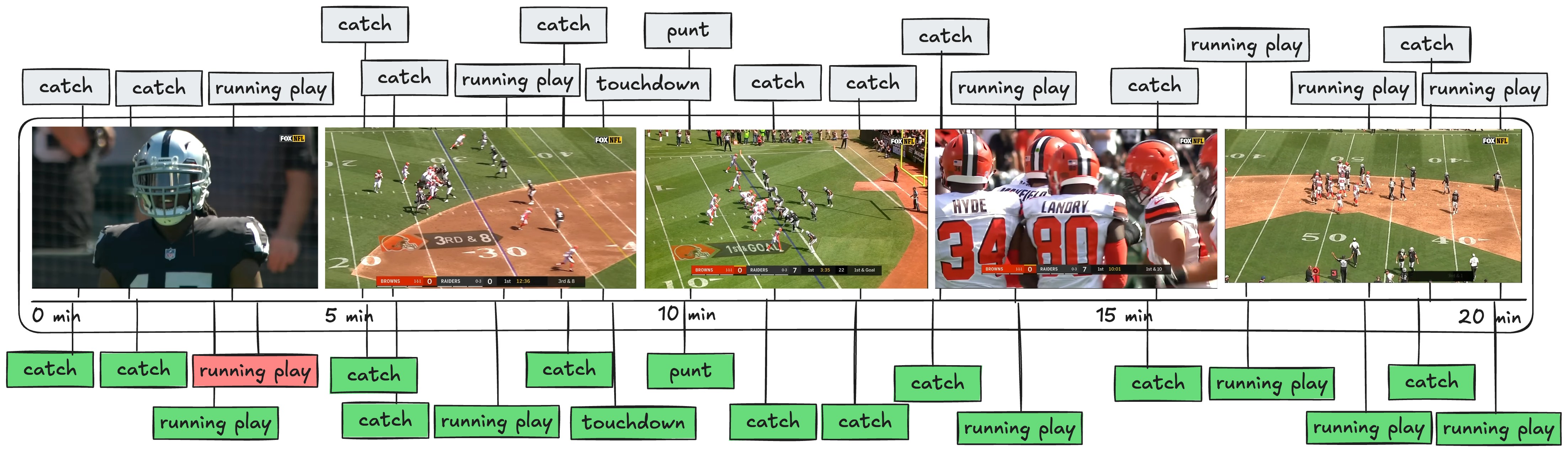
3.1 Aligning Game-Time with Video-Time

To solve this, we utilized the consistent visual feature found in all NFL broadcasts—the on-screen scoreboard. This scoreboard continuously displays vital game information, including scores, current quarter, down and yardage, and crucially, the game clock itself. By extracting this information, we could precisely map the game's official timestamps to corresponding points in the video.

How We Achieved This:

OCR-based Timestamp Extraction: We processed the video using an Optical Character Recognition (OCR) model to detect and extract visible game times from the scoreboard throughout the video.

Frame Sampling Optimization: To optimize efficiency, we sampled just one frame per second (1 fps) for OCR processing. This significantly reduced computational load without compromising the accuracy of the extracted timestamps.

Timestamp Mapping Creation: The OCR results provided an exact correlation between the official game timestamps and the actual runtime of the video. Using this mapping, we segmented the video accurately into individual play-by-play events.

from videodb import SceneExtractionType

# 1 frame per second

scene_collection = video.extract_scenes(

extraction_type=SceneExtractionType.time_based,

extraction_config={"time": 1, "select_frames": ["first"]}

)

print(f"Scene Collection ID: {scene_collection.id}")

# Perform OCR with structured prompt

scene_ocr_results = {}

for scene in scene_collection.scenes:

for frame in scene.frames:

structured_description = frame.describe(

"""Perform OCR to extract the information from the scorebar present.

on the bottom of the image. Output in a structured JSON format:

<team1 name>: <team1 score>, <team2 name>: <team2 score>,

quarter_number: <quarter number>, game_clock: <time left>.""" )

# Save the OCR result with scene start time as the key

scene_ocr_results[scene.start] = structured_description

print(scene_ocr_results)

--------------------------------------------

Example Output:

{

1.0: {"Browns": 0, "Raiders": 0, "quarter_number": 1, "game_clock": "15:00"}

2.0: {"Browns": 0, "Raiders": 0, "quarter_number": 1, "game_clock": "14:59"}

...

}

Integrating Play-by-Play Segmentation with VideoDB

VideoDB effectively supports this customized, non-uniform segmentation approach. We imported our precise timestamp mappings directly into VideoDB, creating accurate and detailed scene indexes seamlessly:

# code snippet for detecting catches from the game footage

# Step 1: Use the stats PDF to filter all play timestamps (game clock) where a catch occurred into `catch_play_scenes` as a list of (start, end) for plays with catches

# Step 2: Map game clocks to video timestamps using OCR outputs

catch_details = []

#iterate over each play

for play_scene in catch_play_scenes:

start_time, end_time = play_scene

#create a new scene object of the play

scene = Scene(

video_id=video.id,

start=start_time,

end=end_time

)

# Call describe with structured prompt to get catch_details

result = scene.describe(

""""This clip contains a catch.

Extract: type of catch,

position of the player who caught the ball,

and whether it was an interception.

Return a structured JSON with keys

{catch_type,player_position,interception}."""

)

catch_details.append({

"scene_start": start_time,

"scene_end": end_time,

"details": result

})

print(catch_details)

--------------------------------------------

Example Output:

[

{

"scene_start": 120.0,

"scene_end": 165.0,

"details": {

"catch_type": "over the shoulder",

"player_position": "centre of the field",

"interception": False

}

...

]

# Do the same for other concepts ( other than catches )

By adopting this precise segmentation strategy, VideoDB enhanced accuracy, dramatically reduced misclassifications, and simplified complex visual analysis tasks, providing unparalleled insights into detailed sports event analysis.

Observations

Evaluation metric

Observation

Hallucination

11.4%

Temporal Context

perfect

Performance on Granular Queries

High

VideoDB Involvement

High

There are no rows in this table

⁠

Approach Comparison

Approach Comparison

Evaluation Metric

Naïve Whole-Video

Uniform Chunks

Play-by-Play

Hallucination

68.1 %

74.2 %

11.4 % ✅

Temporal Context

Poor

Insufficient

Perfect ✅

Granular Queries

Moderate

High ✅

VideoDB Use

Low

Moderate

High ✅

There are no rows in this table

⁠

Key Takeaways

Define Key Sports Concepts:

Clearly outline and specify each concept required for analysis. For example:

Catch (Yes/No)

Running Play (Yes/No)

Scoring Event (Yes/No)

Check Availability of Statistical Data:

Determine if these concepts can be reliably extracted from existing statistical data:

If statistical data is available: use it to isolate specific plays.

If statistical data is not available: directly use the Vision Language Model (VLM) for visual extraction.

Extract Relevant Plays Using Statistical Data:

Use accurate statistical information to isolate relevant video scenes using VideoDB Timeline.

Record timestamps and relevant metadata for these Scenes.

Visual Analysis with VideoDB indexing:

Pass the extracted scenes into the VLM to gather detailed visual insights (e.g., identifying catch types like "overhead" and positions like "near sidelines").

Clearly Structure the Output Data:

Organize the extracted visual information into structured data for clarity and ease of querying. For instance:

[

{

"play_start_time" : 12,

"play_end_time" : 52,

"details": {

"catch": true,

"type": "overhead",

"position": "near sidelines",

"interception" : false,

"running_play": true